Decision tree

I went through a small notebook that trains a DecisionTreeClassifier on the Iris dataset, tunes it with cross-validation, and reads off which features the tree actually relies on. None of the code is long, but every line rests on a piece of maths that is easy to skip past. This post walks through both: what the code does, and why the numbers come out the way they do.

The dataset

The Iris dataset is 150 flowers, split evenly across three species: Iris setosa, Iris versicolor, and Iris virginica 50 rows each. Every flower is described by four measurements, all in centimetres:

import pandas as pd

iris_data = pd.read_csv('./IRIS.csv')
iris_data.head()

   sepal_length  sepal_width  petal_length  petal_width      species
0           5.1          3.5           1.4          0.2  Iris-setosa
1           4.9          3.0           1.4          0.2  Iris-setosa

The label column, species, is text. A decision tree in scikit-learn can technically split on string labels directly, but to keep things explicit I mapped each species to a small integer code:

mapping = {'Iris-setosa': '1', 'Iris-versicolor': '2', 'Iris-virginica': '3'}
iris_data.species = iris_data.species.map(mapping)

The rest of the notebook treats species as the target $y$ and the four measurements as the feature matrix $X$:

X = iris_data.drop('species', axis=1)
y = iris_data['species']

Splitting the data

Before fitting anything, the data is split into a training set and a held-out test set, 80/20:

from sklearn.model_selection import train_test_split

X_train, X_test, y_train, y_test = train_test_split(
    X, y, test_size=0.2, random_state=42
)

With 150 rows total, that is $150 \times 0.2 = 30$ rows reserved for testing and $120$ rows left to train on. random_state=42 just fixes the shuffle so the split is reproducible.

What a decision tree is actually doing

A classification tree makes every decision by asking a single yes/no question about one feature at a time "is petal_length $\le 2.45$?" and routing the sample left or right depending on the answer. Training the tree means choosing, at every node, which feature and which threshold to ask about.

The tree does this by trying to make each resulting group as pure as possible, i.e. as dominated by a single species as it can get. Purity at a node $t$ is measured with the Gini impurity:

where $p_k$ is the fraction of samples at node $t$ that belong to class $k$, and $K$ is the number of classes (here, $K = 3$). A node with only one species present has $Gini(t) = 0$; a node split evenly across all three species has the impurity at its maximum. (Setting criterion='entropy' swaps this for $H(t) = -\sum_k p_k \log_2 p_k$, which behaves similarly but is on a different scale the notebook leaves the default, Gini, in place.)

For a candidate split $s$ that divides node $t$ into a left child $t_L$ and a right child $t_R$, the tree scores it by how much impurity that split removes:

where $N_t$ is the number of samples at $t$, and $N_L$, $N_R$ are how many of those went left and right. At every node, the tree scans every feature and every possible threshold, and keeps whichever split maximises $\Delta(s, t)$. It repeats this recursively on each child until nodes are pure, or until some stopping rule (max_depth, min_samples_leaf, and so on) kicks in.

from sklearn.tree import DecisionTreeClassifier

clf = DecisionTreeClassifier()
clf.fit(X_train, y_train)

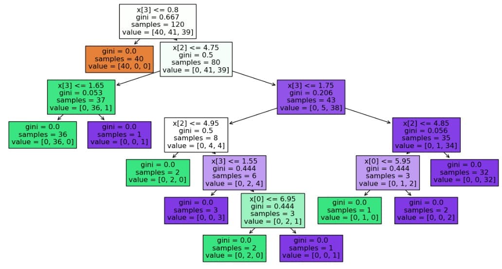
With no max_depth set, this tree grows until every leaf is pure it will happily memorise noise in the training set if the data allows it. Plotting it makes that literal:

from sklearn import tree
import matplotlib.pyplot as plt

plt.figure(figsize=(15, 8))
tree.plot_tree(clf, filled=True)

Choosing a depth with cross-validation

An unconstrained tree overfits. Instead of guessing max_depth, the notebook searches over a small grid of values and picks the one that generalises best, using 5-fold cross-validation:

from sklearn.model_selection import GridSearchCV, KFold

kf = KFold(random_state=42, shuffle=True, n_splits=5)
params_grid = {'max_depth': [1, 2, 3, 4, 5, 6]}
grid_cv = GridSearchCV(clf, params_grid, cv=kf)
grid_cv.fit(X_train, y_train)

$K$-fold cross-validation with $K = 5$ works like this: the 120 training rows are shuffled and cut into 5 equal folds. For each candidate max_depth, the tree is trained 5 times, each time on 4 folds ($\approx 96$ rows) and validated on the 1 remaining fold ($\approx 24$ rows). The 5 validation scores are averaged:

where $f_d^{(-i)}$ is a tree of depth $d$ trained on every fold except fold $i$. GridSearchCV repeats this for every value in params_grid and keeps whichever depth scores highest on average — here, that turned out to be:

print(grid_cv.best_params_)
# {'max_depth': 3}

A depth of 3 is small enough to avoid memorising the training set, while still letting the tree separate all three species Iris is an easy dataset in that sense, since setosa is linearly separable from the other two on petal measurements alone, and versicolor/virginica need only a couple more splits.

Reading feature importance

Once the tree is trained, it's possible to ask which features it actually relied on:

clf.feature_importances_
# array([0.03334028, 0.        , 0.38926487, 0.57739485])

For a single tree, scikit-learn computes the importance of feature $f$ by summing the impurity decrease at every node that split on $f$, weighted by how much of the data passed through that node, then normalising so the importances across all features sum to 1:

A feature the tree never splits on contributes zero, which is exactly what happens to sepal_width here. Sorting the result makes the ranking easy to read:

feature_names = X.columns
feature_importance = (
    pd.DataFrame(clf.feature_importances_, index=feature_names)
    .sort_values(0, ascending=False)
)
feature_importance

                     0
petal_width   0.577395
petal_length  0.389265
sepal_length  0.033340
sepal_width   0.000000

Petal measurements alone account for over 96% of the tree's decisions, which lines up with the well-known fact about this dataset: petal size separates the three Iris species far more cleanly than sepal size does. Dropping the zero-importance row and plotting the rest makes the point visually:

feature_importance = feature_importance[feature_importance.iloc[:, 0] > 0]
feature_importance.plot(kind='bar')

What this leaves out

The notebook stops at feature importance it never scores the tuned tree on the held-out X_test/y_test set, so there's no final accuracy number here, only the cross-validated score used to pick max_depth. That's the natural next step: refit grid_cv.best_estimator_ and check accuracy_score on the 30 rows that were set aside at the very start.